Analyzing Switch Mode Power Supply Loop Gain

In the interest of stability, the open loop gain of a negative feedback system operating in closed loop should fall below unity with increasing frequency before too much phase shift occurs unless your aim actually is to make an oscillator[1]. This idea can be applied to the stability analysis of a Switch Mode Power Supply (SMPS). Even though an SMPS is an intrinsically non-linear circuit with no small-signal linear equivalent circuit, there typically is an analog feedback loop operating on the filtered, switched output.

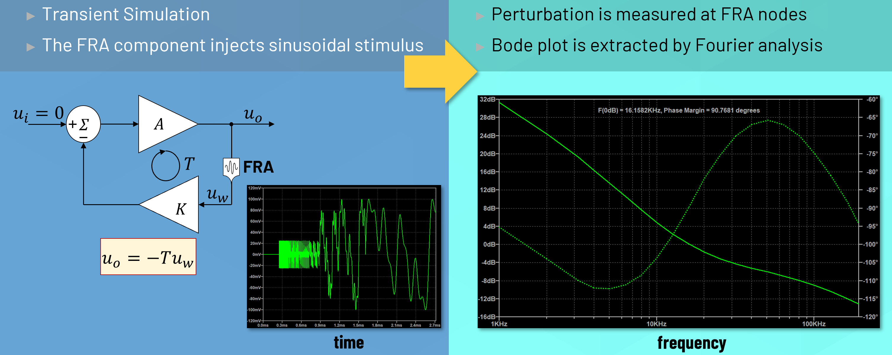
The technique of using injected test signals and Fourier analysis is called Frequency Response Analysis(FRA). LTspice provides integrated FRA functionality. The LTspice FRA employs the voltage-only version of Middlebrook's method[2], applicable when the feedback loop has a point of low impedance driving high impedance, which is generally the case for a SMPS since the power supply output drives an error amplifier input.

Several FRA example circuits are provided with LTspice. To open these, choose File > Open Examples, and navigate to the schematics located in Educational\FRA\

The FRA is a specialized time-domain transient simulation. During the analysis, the FRA component injects sinusoidal stimulus into the circuit, and measures the response. A Bode plot is extracted by Fourier analysis.

FRA Settings

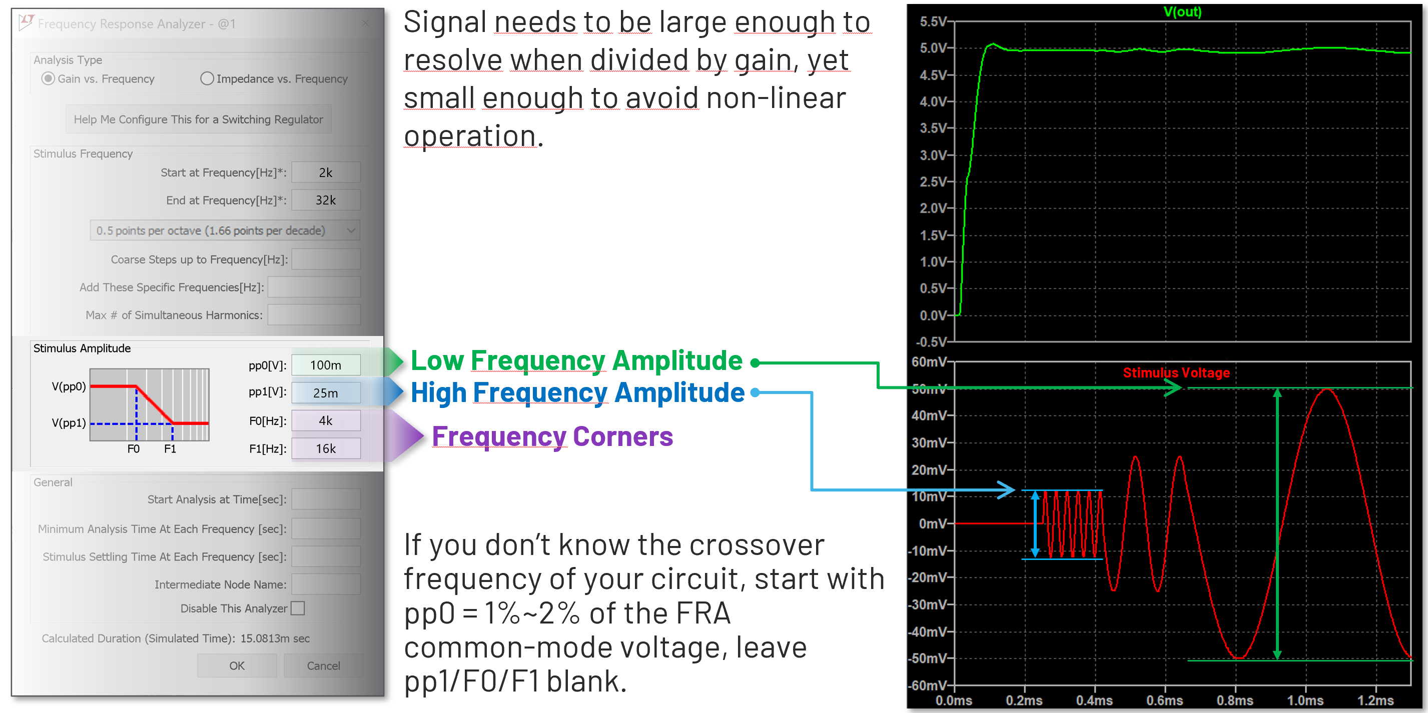
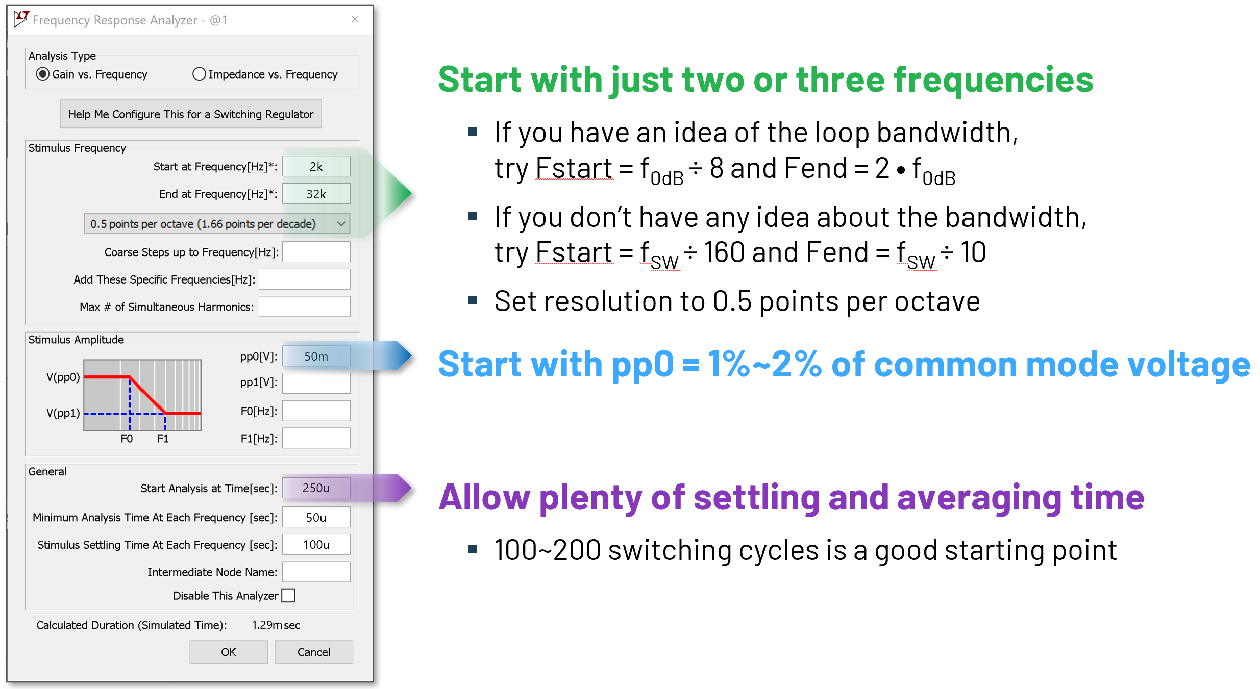
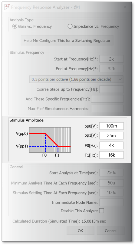
The stimulus is controlled by FRA component. Right-clicking on the FRA component brings up the dialog shown in the images below.

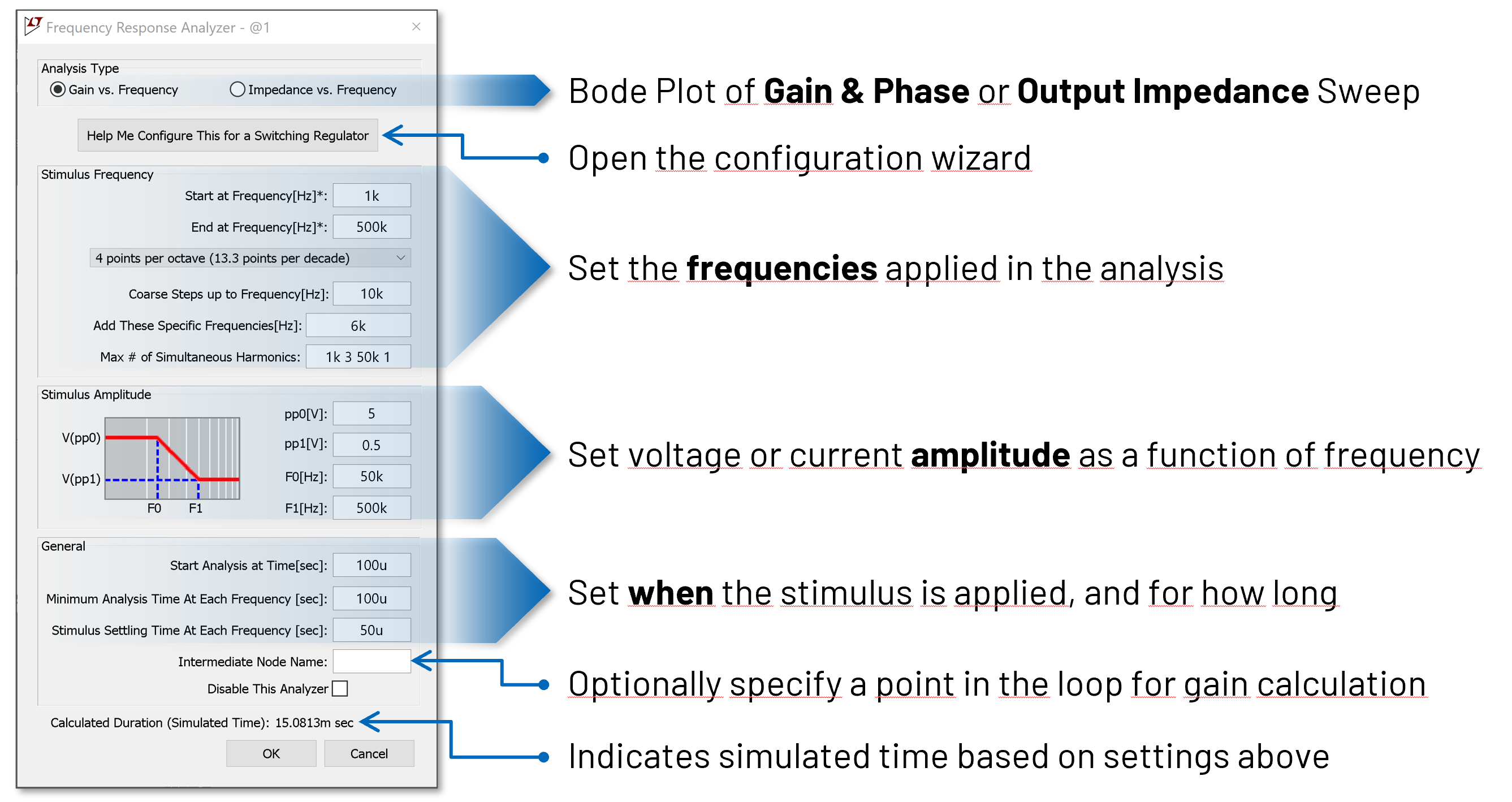
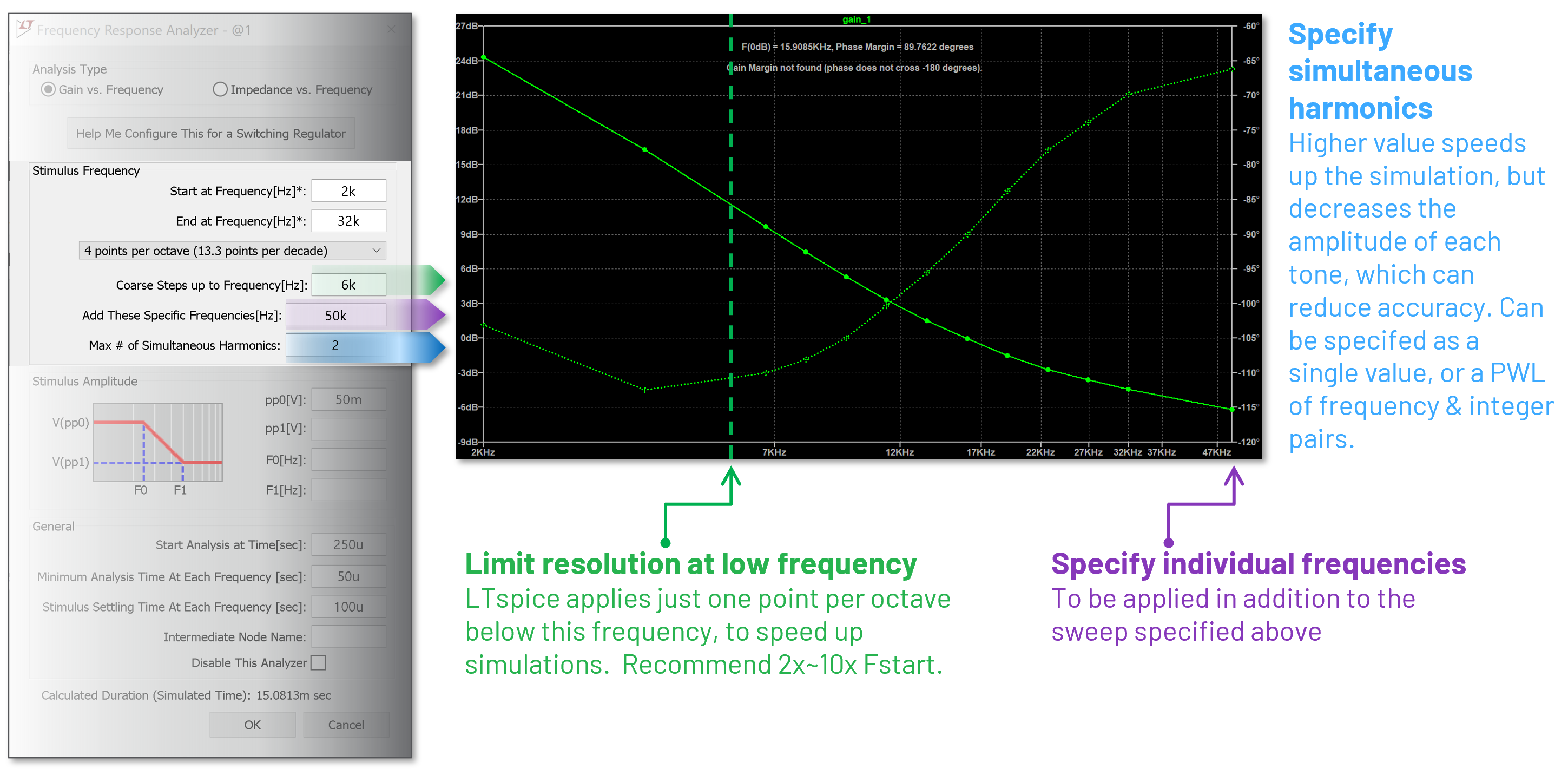
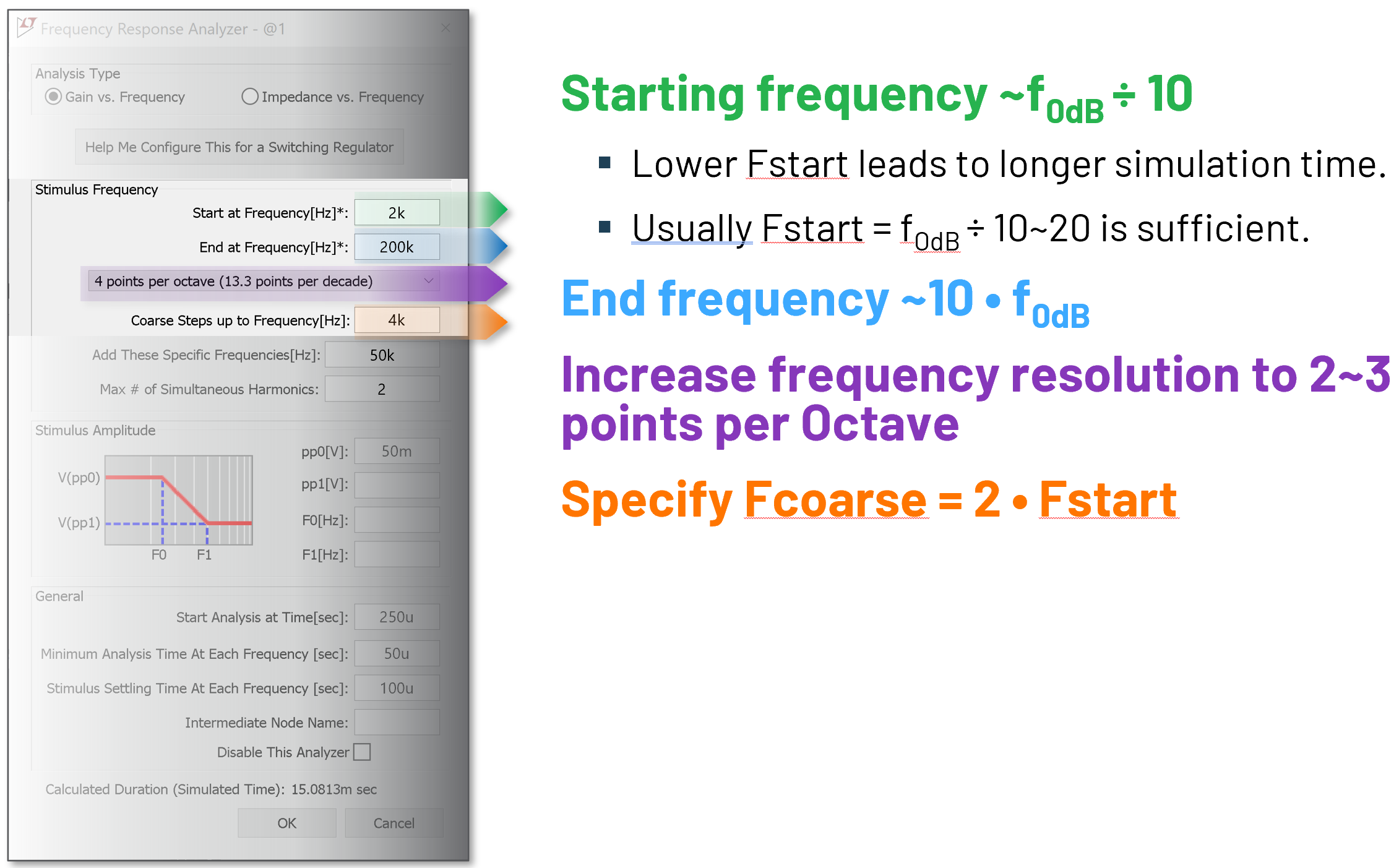
The images below demonstrate the effect of stimulus frequency parameters:

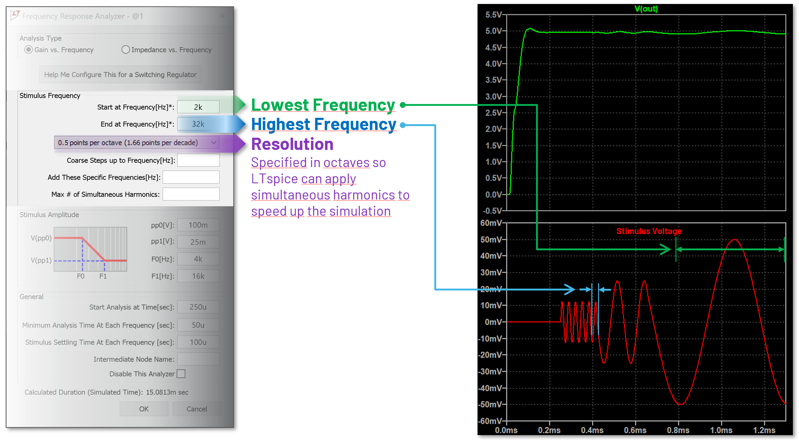
The image below demonstrates the effect of the stimulus amplitude parameters:

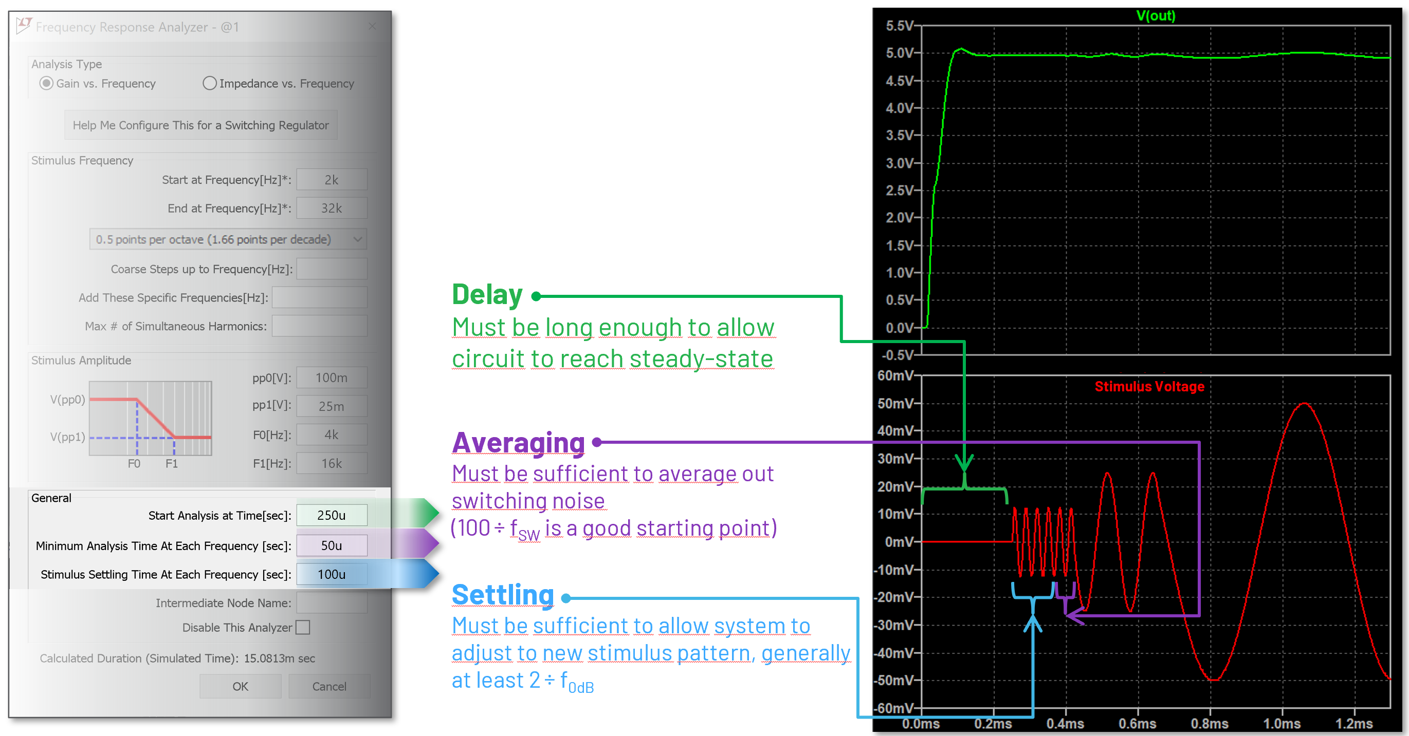
The General parameters control when the stimulus is applied, as shown below:

Step-by-step how-to

This section describes a procedure for setting up the FRA to efficiently provide meaningful results for a SMPS circuit, using the LT8609 as an example.

The overall procedure is as follows:

1. Investigate and prepare the circuit

2. Break the loop

3. Initial FRA setup

4. Inspect the FRA transient waveforms

5. Initial Bode Analysis

6. Optimize the stimulus

7. Extend to more frequencies

9. Speed up the analysis

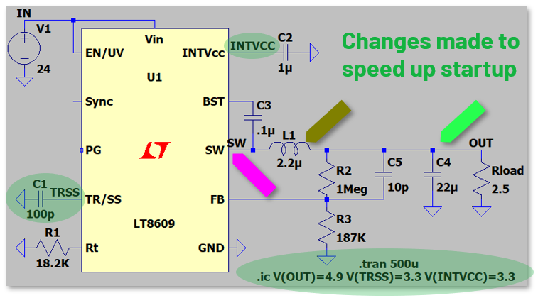
1. Start with a basic startup transient simulation of the SMPS.

* Plot and examine the switch node, inductor current, and output voltage.

* Consider speeding up the time required to settle to steady-state, for example, by applying initial conditions, reducing the soft-start cap. See the article https://www.analog.com/en/technical-articles/ltspice-speed-up-your-simulations.html

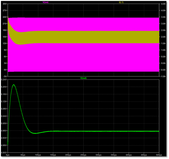
Make note of:

* Time required to settle to steady-state (<250us in this example)

* Final output voltage (~5V in this example)

* Switching frequency (~2MHz in this example)

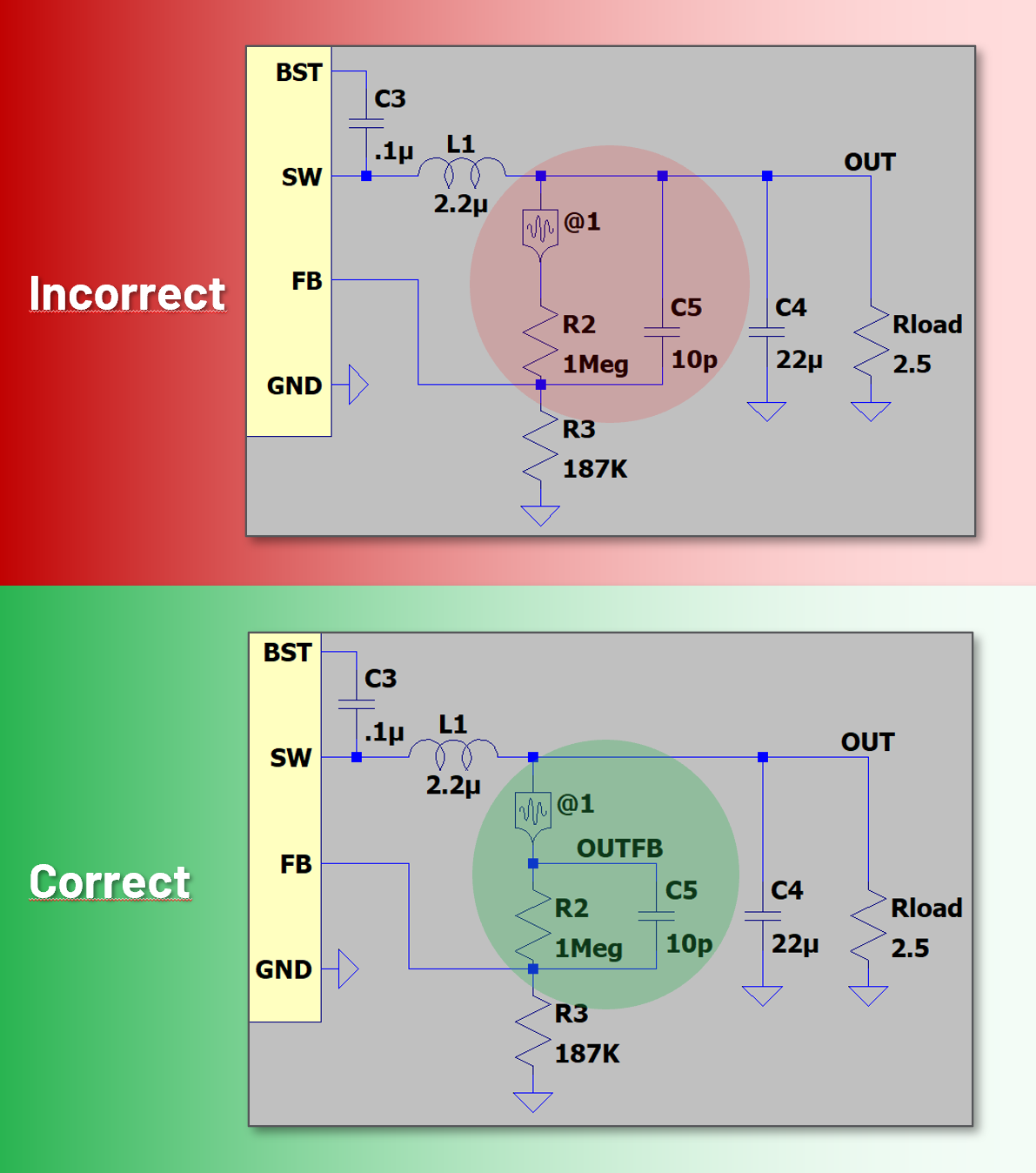
2. Break the loop and insert the FRA component

Criteria:

The FRA component must interrupt all feedback paths

The FRA component must point from lower impedance (flat side) to higher impedance (pointy side)

3. Initial FRA Setup - Exploratory

* Start with just two or three frequencies

- If you have an idea of the loop bandwidth, start with Fstart=f0dB / 8 and Fend=2*f0dB

- If you don't have any idea what the bandwidth might be, start with Fstart=fsw/160 and Fend=fsw/10

- Set the resolution to 0.5 points per octave

* Start with pp0=1%~2% of the common-mode voltage at the FRA component.

* Allow plenty of settling and averaging time. 100~200 switching cycles is a good starting point.

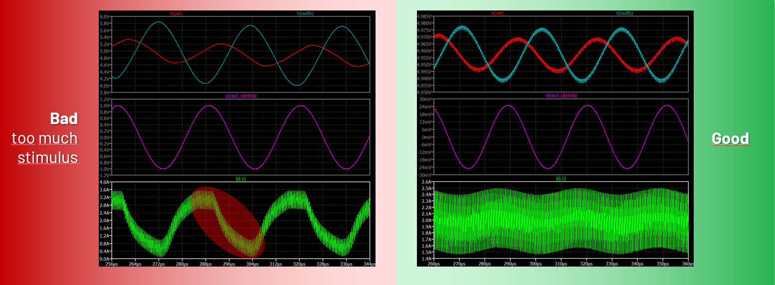
4. Run the simulation and inspect the FRA transient waveforms.

Plot and examine:

- Voltage at both FRA terminals

- Inductor current

- Control voltage (if available)

Ideally, sinusoidal pattern should be evident and symmetric.

- Look for signs of non-linearity, indicating stimulus amplitude too large

- Note that there are discontinuities when the frequency changes – these are expected

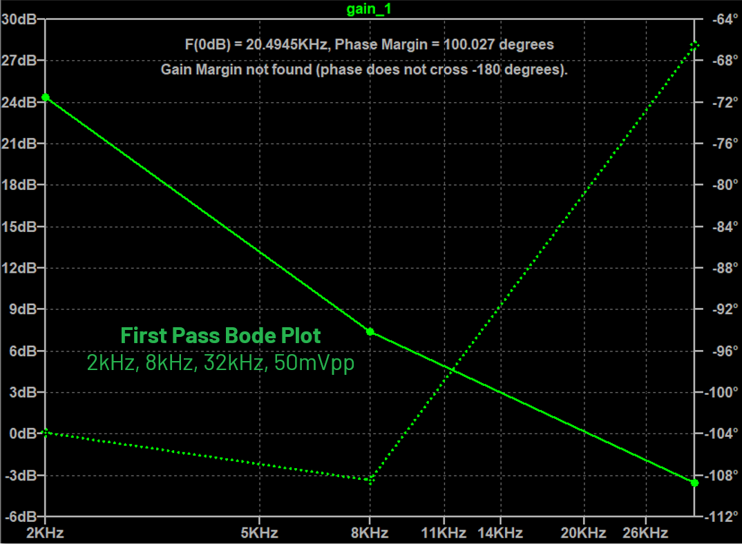
5. Initial Bode Plot Analysis

* Find f0dB

* Adjust Fstart and Fend

- Fstart = f0dB ÷ 8

- Fend = 2 • f0dB

* Re-run FRA

6. Adjust stimulus amplitude

* Specify frequency dependance

- Need more signal at lower frequency due to high gain

- Need less signal at higher frequency to avoid non-linear effects

* A good starting point is:

pp0 = VCM ÷ 25~50

pp1 = pp0 ÷ 4

F0 = f0dB ÷ 4

F1 = f0dB

* After adjusting the stimulus, re-run the simulation until satisfied with the transient behavior (as in step 4) and the 3-point Bode plot.

- Increase amplitude up to perhaps 3~5% of VCM, reducing if asymmetry or non-linearity becomes apparent

- If, as you are increasing the amplitude, non-linearity becomes evident yet the stimulus is still not apparent in waveforms, reduce stimulus amplitude to achieve linear operation, and increase Minimum Analysis Time At Each Frequency (Tavgmin), for example ~1000 ÷ fSW, to allow LTspice to resolve the signal.

- Note that phase tends to be more sensitive to errors than gain

- Adjust and re-run FRA until satisfied with the transient and Bode

7. Add more frequencies

* Starting frequency ~f0dB ÷ 10

-Lower Fstart leads to longer simulation time.

-Usually Fstart = f0dB ÷ 10~20 is sufficient.

* End frequency ~10 • f0dB

* Increase frequency resolution to 2~3 points per Octave

* Specify Fcoarse = 2 • Fstart

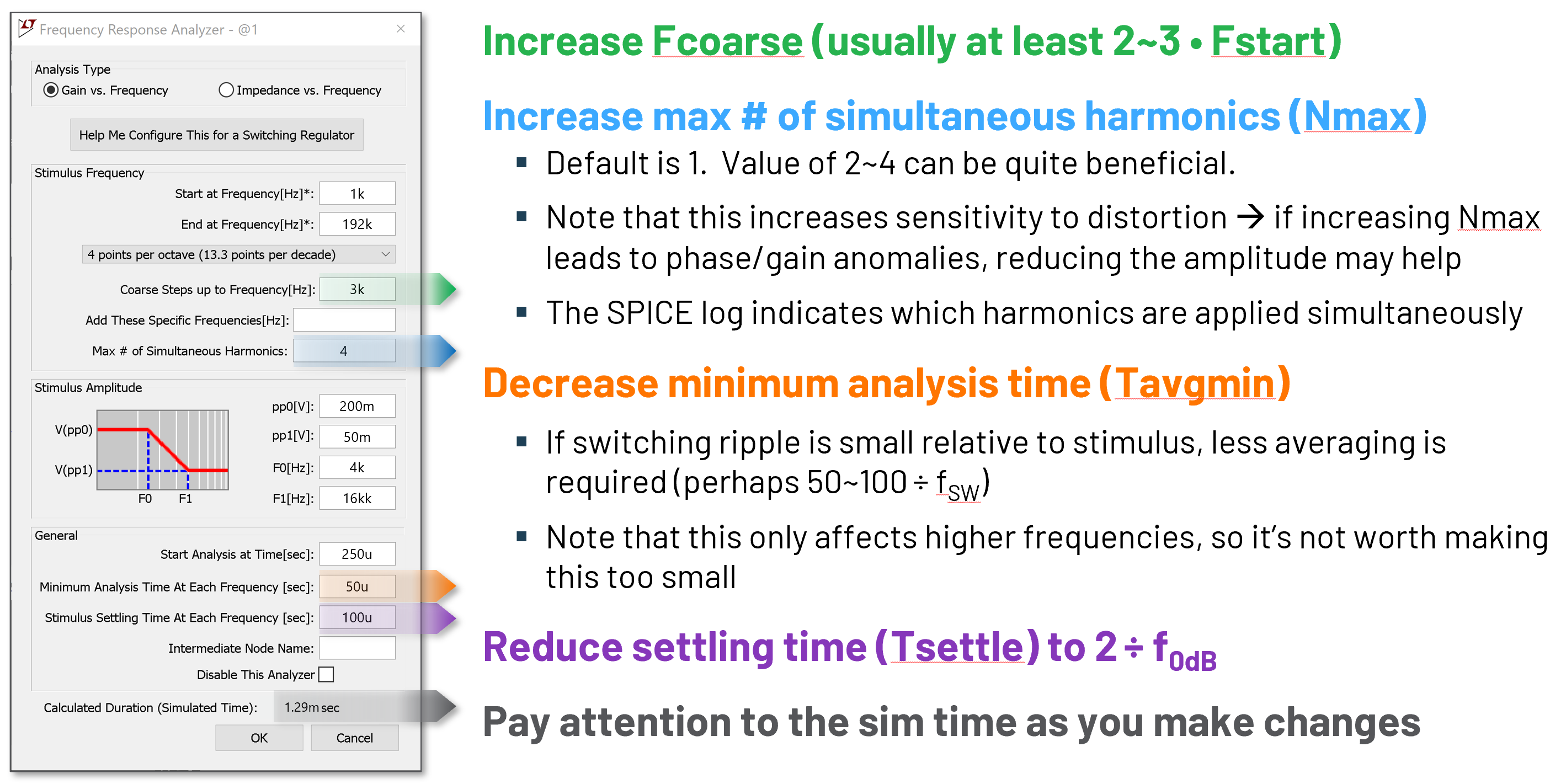
8. (Optional) Speed up the FRA

* If you plan to run further simulations of this circuit, you may choose to adjust the settings to reduce the simulation time. Below are some possible adjustments that can speed up the FRA. Try these incrementally and analyze the simulation results as you proceed, comparing to the previous results to ensure the changes are not adversely affecting the quality of the analysis.

1] The discussion is restricted to minimum-phase systems.

2] R. David Middlebrook, "Measurement of Loop Gain in Feedback Systems", International Journal of Electronics (vol 38, no. 4, pages 485-512, April 1975).